Exploring Craigslist Musicians Communities

In addition to data science, my other passion is playing music. When I would travel around to different clients as a consultant, I usually found myself in new cities yearning to play with other musicians to learn new guitar techniques, cover my favorite songs, or just jam and create original material. In order to connect with other musicians who shared these interests, I relied heavily on responding to the “musicians” posts on Craigslist. After years of using this service I have found that people post for variety of reasons, and sometimes the posts stray away from the express purpose of connecting musicians to each other, e.g. posts about selling gear, studios for rent, a critique of a newly released album. For me, avoiding these posts was fairly easy by using keyword searches. If I wanted to find somebody who wanted to play aggressive and hook-driven punk music, I could just enter searches for “Ramones”, “Ty Segall”, and “Green Day”, and usually I will find someone who has listed one or more of those bands as influences.

However, when embarking on my fourth project at Metis, I wanted to use Craigslist to reflect what different musician communities value in aggregate. Instead of finding people with my specific interests, I was more interested in analyzing the posts’ text to uncover sub-communities of Craigslist “musicians” users to learn more about the poster’s motivations for putting out ads, where these different motivations cluster in major U.S. cities, and perhaps learn more about these poster’s tendencies. In order to accomplish these tasks I decided to use topic modeling to categorize the types of posts on Craigslist, and then build a Flask application to visualize how these categories change across different cities.

Data Acquisition

After getting some test data from https://newyork.craigslist.org/search/muc, I learned that to scrape every post on every Craigslist musicians board is very time-consuming due to the volume of posts. Because I had a week and a half until I had to present my findings and my web app to my Metis cohort, I decided to limit the scope of my data to only those sites which had over 300 posts at the time I scraped them. I created a Scrapy spider to crawl https://www.craigslist.org/about/sites, to find the 45 musicians sites that met this requirement, and then scraped each post on each of the sites for the following information:

• post title text
• post body text
• url of the post (sites on Craigslist are organized by geographic area)
• latitude and logitude of the post (if the post was geo-tagged)

Cleaning and Preprocessing

When I first got the data, I decided to do some broad cleansing of the text in each post:

• removing post metadata created by Craigslist
• removing urls
• removing stopwords from the NLTK corpus module
• Applying NLTK’s implementation of a Porter Stemmer (stemming breaks down words to their root in order to make uniform different words with semantic similarities, e.g. worked and working are transformed to work).

In order to feed this data into a machine learning model, I transformed the cleaned text into a TF-IDF matrix via scikit-learn’s implementation of TfidfVectorizer using unigrams and bigrams. TF-IDF stands for “term frequency, inverse document frequency” and is a commonly used method to vectorize raw text based on the count of the terms in a text document divided by the number of documents in which the term appears in the entire text corpus. The idea here is to keep track of word counts in a given document (i.e. a Craigslist post) that describe the content of the document (e.g. bassist, touring, electric) while penalizing those words which appear too frequently across all documents and do not necessarily give us information on the margin (e.g. music, search, rhythm). “Unigrams” and “bigrams” refer to the tokenization of words into one-word and two-word terms. These terms capture more contextual information about our text (e.g. professional vocalist versus novice vocalist). My TF-IDF matrix can be thought of as a “document-term” matrix which consists of ~20,000 rows (each representing a Craigslist post) and ~600,000 columns each representing a unique unigram or bigram. The values of this table correspond to a given term”s TF-IDF score in a given post.

Topic Modeling

I wanted to see if I could extract any meaningful topics out of my corpus using Non-Negative Matrix Factorization (NMF). NMF is a decomposition technique which, given a n x m matrix Z and k-dimensional features, will create two smaller matrices, X and Y, of sizes n x k and m x k respectively. NMF creates these two smaller matrices with two goals: (1) No values in X or Y can be negative, and (2) X x Y^T is approximately equal to Z.

Using sklearn.decomposition.NMF, I decomposed my TF-IDF matrix into a “term-feature” matrix and a “feature-document” matrix. For this project I chose 18 dimensional features which represent the number of topics in my corpus of posts. After some trial-and-error I found that 18 was a good value because it yielded the most interpretable topics. So how did I go about interpreting these topics? This was a two-step process:

1. Term evaluation

I sorted each feature in my term-feature matrix by the ten terms with the highest weights to get a summary of which terms are the focus of my topics. For example, here are the top ten words for topics 1 and 2:

Rank	Topic 1	Topic 2
1	record	lesson
2	studio	teach
3	record studio	student
4	produce	piano
5	engineer	teacher
6	session	learn
7	artist	drum
8	hr	guitar lesson
9	pro	guitar
10	product	hour

Looking at these terms leads me to believe that topic 1 is likely filled with posts about studio and producer services for artists, and topic 2 is likely ads for music teachers (primarily for piano, guitar and drums). But how do we confirm this?

2. Document inspection

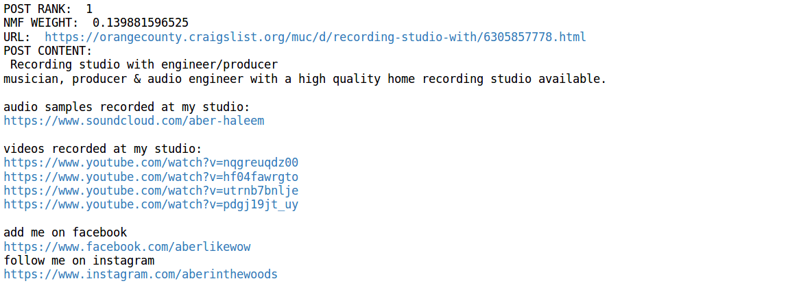
To get better context for my topics I sorted each feature of my feature-document matrix by the ten documents with the highest weights. Here is an example of the most heavily weighted posts for topics 1 and 2:

Topic 1:

Topic 2:

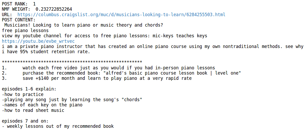
These posts seem to confirm my initial hypothesis. By repeating this process for each topic and checking the top ten posts in each group, I can more confidently apply a label to each topic, which I have listed below.

Topic	Description
0	New Music Projects
1	Studio Services
2	Teachers
3	Bassists
4	Drummers
5	Music for Your Event!
6	Metalheads
7	Rehearsal Spaces
8	En Espanol
9	Cover Bands
10	Producer/Ghostwriter Ad Spam
11	Mixing and Mastering
12	Guitarists
13	Classic Rock
14	Church
15	Music Videos
16	Singer/Songwriters
17	Open Mics and Jams

Key Findings

Scraping, cleaning, and modeling the data was quite an effort in itself. But now that I had my text categorized into topics was there anything I could glean from it?

Spam detection

Here is a breakdown of the prevalence of posts across my topics:

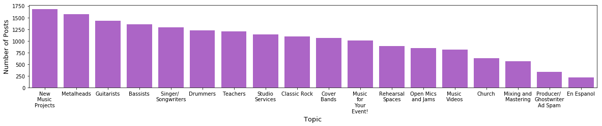
Upon my first run of NMF and the creation of this chart, the label “Producer/Ghostwriter Ad Spam” had far more posts than it does presently. When I took a closer look at the documents with that label, I found very obvious instances of posts that were duplicated by the same source across different craigslist sites. The two posts below are good examples:

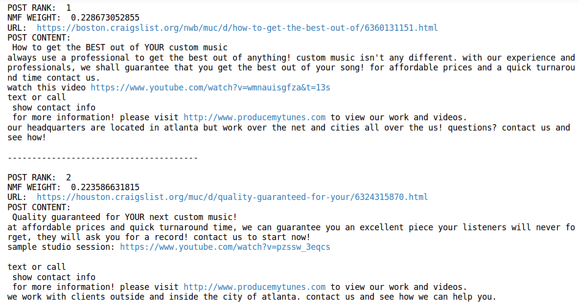
The ads promoting www.producemytunes.com and a few other spammers were very prominent in my dataset. These ads are clearly from the same source but the spammers took care to switch up the language in most their posts (probably to avoid being flagged as spam by site moderators). For purposes of creating my Flask application, I did not want these duplicate ads taking up space and diluting the topic space for a given geographic area so I had to find a way to get rid of them. However, the problem of numerous ads from the same source was more rampant than I thought and could not be overcome by eliminating certain ads using pattern matching.

In order to weed out these duplicates I had to do some additional preprocessing. My solution consisted of vectorizing my posts back in the cleaning stage using a CountVectorizer and computing the cosine similarities between these vectors. The CountVectorizer serves the same purpose as the TfidfVectorizer, but instead of penalizing terms for being too frequent across the corpus it just counts all instances of all terms in each document. Cosine similarity measures the cosine of the angle between any two given document vectors. This is a useful way to measure the distance between two vectors in a high-dimensional space, such as two texts with many term dimensions. If the cosine similarity between two of my document vectors is 1, this means they are identical documents; if the cosine distance is 0, they share none of the same terms. I settled on a fairly high threshold of 0.98, iterated through my vectorized posts, computed the cosine similarities of each post to every other post, and eliminated any posts in my dataset that exceeded the threshold (sparing the comparison post in each iteration). This process led me to eliminate 1,140 duplicate posts from my dataset.

Uncovering possible musical genre bias

Consider the chart below. It is the same one as above but I have added in the top ten terms associated with each topic.

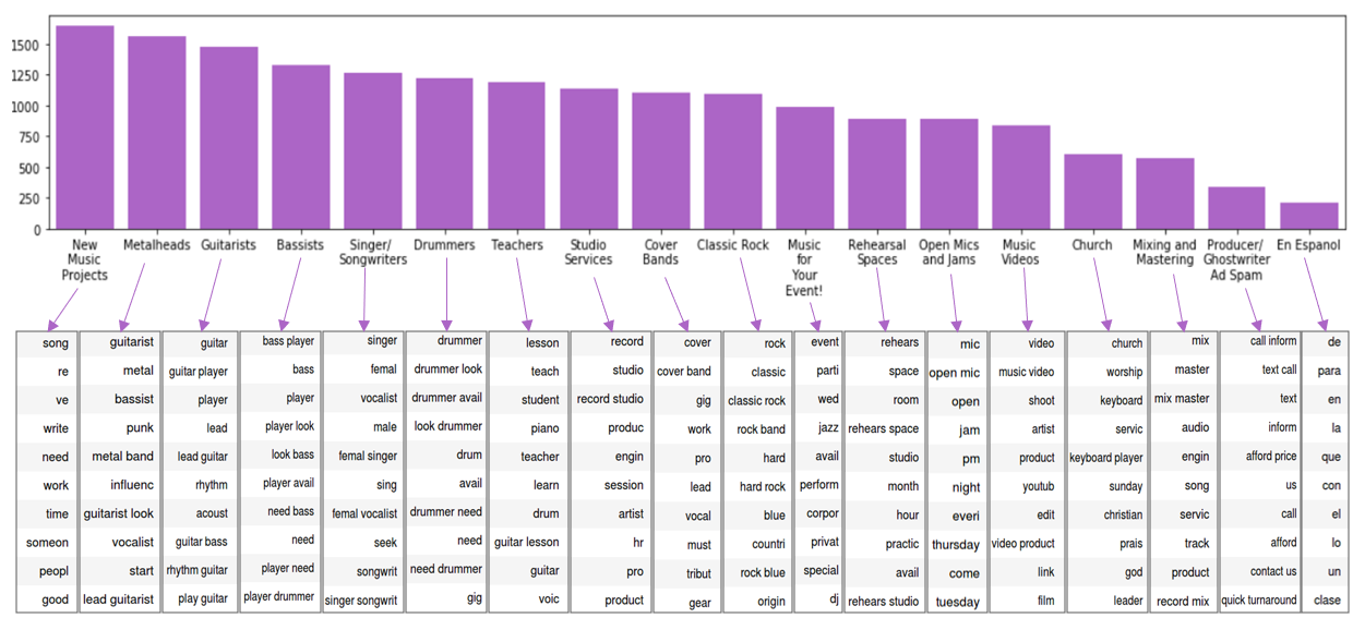
Being someone who has found many musicians willing to play punk rock through Craigslist, it was no surprise to me that many of the terms seemed pointed at the “rock” genre. However, it was surprising to see no evidence of other popular genres such as “hip-hop” or “electronic/EDM music”. Does this point to an over-representation of rockers in my dataset? To answer this question I decided to run genre-specific keyword searches through all of my posts to find any direct mentions of specific genres and/or their associated sub-genres. I converted a pre-defined music genre taxonomy from this website to my own python dictionary and counted the number of matches for a given master genre. The chart below shows the proportion of posts in which a given genre keyword appears.

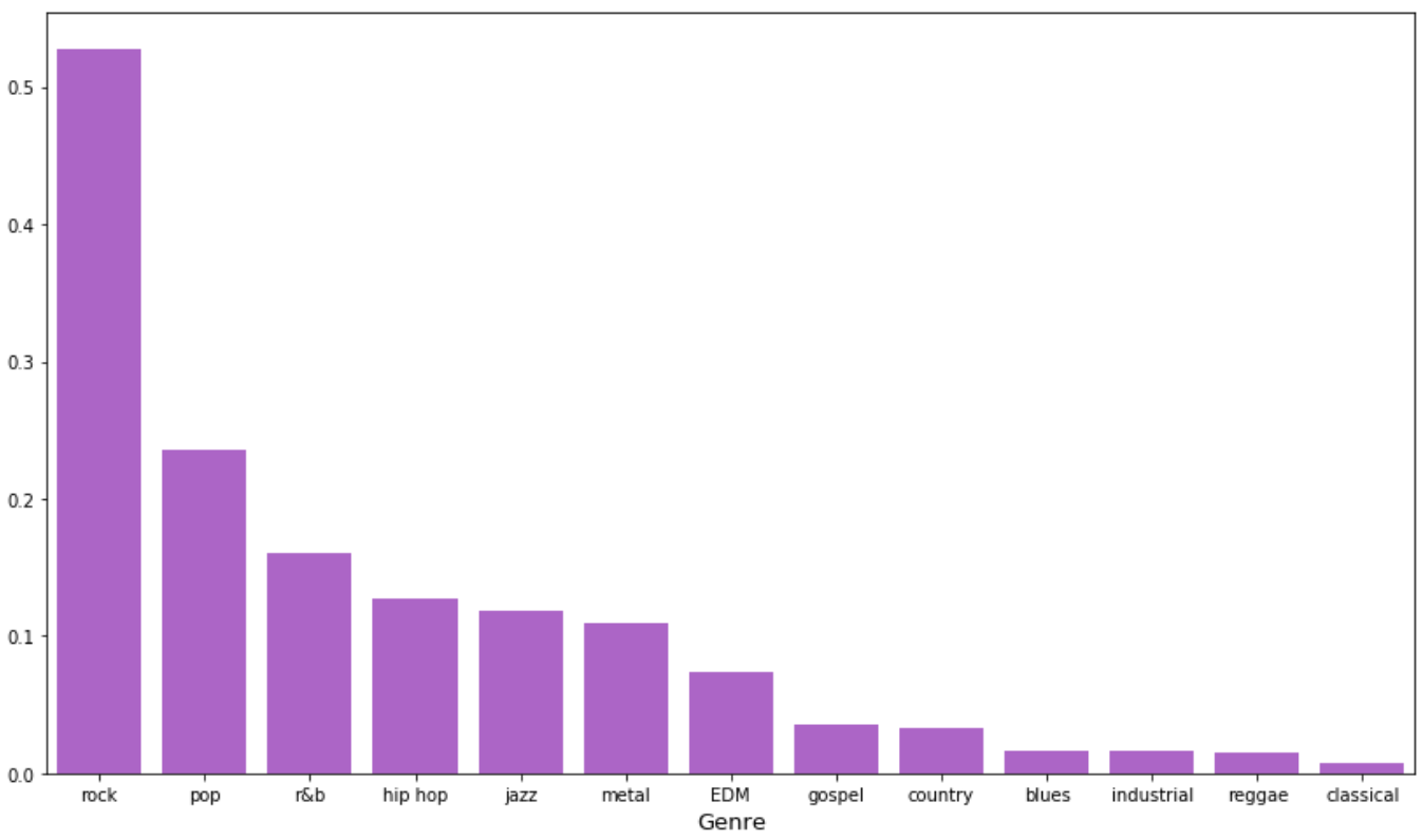
It appears that “rock” shows up in over 50% of the posts in my dataset–more than double that of any other genre. While this finding combined with the rock-centered NMF topics is compelling evidence of bias amongst Craigslist users, consider that this data is from one specific point in time.

Visual clusters

The plot below is a projection of my document vectors which I created using a technique called t-SNE. t-SNE compresses the 18-dimensional document vectors into 2-dimensional coordinates which I can plot to see the spatial separability between my topic clusters. In order to clear up some of the clusters for this plot I had to remove 3,446 of the 18,366 data points by filtering out any document vectors that did not have a maximum topic weight of over 0.02.

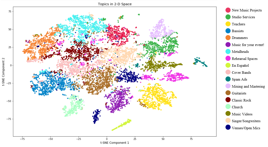
The t-SNE plot shows some spatial separability between the 18 topics, but the fact that I had to remove roughly 20% of the data to get this view suggests that this NMF model has not learned everything there is to learn about this data in order to confidently place each and every post into its own bucket. I want to end with this plot as it highlights some possible improvements I can make to this project in the future which include:

• Applying clustering algorithms to assign posts to the NMF-generated features (I tried using K-Means for this purpose but the clusters I got from choosing the maximum topic weights made more sense to me).
• Experimenting with other algorithms on my data to do topic modeling, such as Latent Dirichlet Allocation or Latent Semantic Analysis.
• Trying different text preprocessing steps, such as lemmatization instead of stemming.

Flask Application

I mentioned above that I created a Flask app to visualize my NMF-generated topics. The app is currently hosted on AWS and can be visited at this link. I used dc.js and Leaflet to generate the charts and map respectively. Underlying the charts and map is a set of crossfilter dimensions which allow objects to track the same data and filter each other (i.e. zooming in/out on the map automatically re-adjusts the bar charts and selecting/de-selecting bars on the charts filters both charts and the map).

The scripts for this project can be found here.